Tutorial
A CAMFR simulation is a Python script: it sets global parameters, defines
materials and waveguides, combines them into structures and asks for modes,
scattering matrices or fields. The examples below run as they are; the
examples/tutorial
directory has longer ones.
from camfr import * imports CAMFR and, as it always has, the NumPy namespace
(zeros, arange, …). import camfr works as well.
Modes of a slab waveguide
from camfr import *

set_lambda(1.0)            # wavelength; lengths use the same unit (µm)
set_N(20)                  # number of modes in the expansion
set_polarisation(TE)

GaAs = Material(3.5)       # refractive index; loss is a negative imaginary part
air  = Material(1.0)

slab = Slab(air(2) + GaAs(0.5) + air(2))
slab.calc()

for i in range(3):
    print(i, slab.mode(i).n_eff())
0 (3.3979427355559184+0j)
1 (3.076686613678061+0j)
2 (2.4773733415055106+0j)
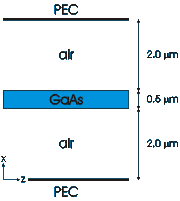
Calling a material with a thickness, GaAs(0.5), gives a layer; + stacks
layers along x, from x = 0. The slab lies between two perfectly conducting
walls (figure below); the modes propagate along z.
slab.mode(i) returns a Mode, with n_eff(), kz() and
field(Coord(x, y, z)). A Field has the components E1(),
E2(), Ez(), H1(), H2(), Hz(), where 1 and 2 are x and y:
f = slab.mode(0).field(Coord(2.25, 0, 0))   # centre of the core
print(f.E2())
Scattering by a stack
A Stack joins waveguide sections along z. Calling a
waveguide with a length gives a section; the first and last sections are
semi-infinite, so their lengths only mark the reference planes.
space = Slab(air(4.5))

for L in [0.02, 0.04, 0.06, 0.08]:
    stack = Stack(space(0) + slab(L) + space(0))
    stack.calc()
    print(f"{L:.2f}  {abs(stack.R12(0, 0)):.4f}")
0.02  0.0365
0.04  0.0982
0.06  0.1954
0.08  0.3129
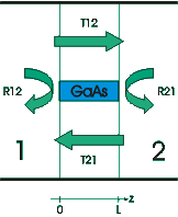
stack.calc() computes the scattering matrices. R12 and T12 are the
reflection and transmission matrices for light incident from the left (medium
1), R21 and T21 from the right; R12(i, j) is the reflection from mode j
into mode i.
(The warning “mode close to cutoff” printed here concerns the closed air box: at this wavelength one of its modes is exactly at cutoff. Harmless in this example, but see Solvers and settings.)
Fields in a stack
To see fields, set an incident field (mode amplitudes, one per mode) and
evaluate stack.field(Coord(x, y, z)). This example shoots the fundamental
mode across a 1 µm air gap. The claddings get a PML, so that light escaping
from the waveguide is absorbed instead of reflected by the walls:
from camfr import *
import matplotlib.pyplot as plt

set_lambda(1.0)
set_N(40)
set_polarisation(TE)
set_lower_PML(-0.1)
set_upper_PML(-0.1)

GaAs = Material(3.5)
air  = Material(1.0)

slab  = Slab(air(2) + GaAs(0.5) + air(2))
space = Slab(air(4.5))

stack = Stack(slab(1) + space(1) + slab(1))

inc = zeros(N())
inc[0] = 1                    # fundamental mode incident from the left
stack.set_inc_field(inc)
stack.calc()

print(abs(stack.R12(0, 0))**2, abs(stack.T12(0, 0))**2)   # 0.356 0.115

x = arange(0, 4.5, 0.02)
z = arange(0, 3, 0.02)
E = array([[abs(stack.field(Coord(xi, 0, zi)).E2()) for zi in z] for xi in x])

plt.imshow(E, origin="lower", extent=(z[0], z[-1], x[0], x[-1]), cmap="magma")
plt.xlabel("z (µm)")
plt.ylabel("x (µm)")
plt.colorbar(label="|E$_y$|")
plt.show()
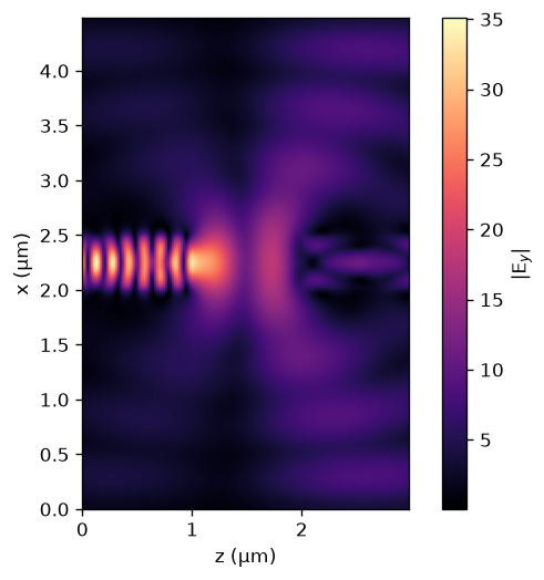
About 36 % of the power is reflected into the fundamental mode, 12 % is
transmitted into it, and the rest radiates away or couples to other modes.
CAMFR’s own plotting helpers do the same in one call
(stack.plot_field(lambda f: abs(f.E2()), x, z)), or interactively
(stack.plot()).
A 3D waveguide: silicon wire
A Section is a 2D cross-section: slabs (layered along y)
joined along x. This is a 500 × 220 nm silicon wire in oxide at 1550 nm:
from camfr import *

set_lambda(1.55)
set_N(3)                      # modes wanted

Si   = Material(3.476)
SiO2 = Material(1.444)

set_section_solver(L)
set_mode_correction(full)
for set_PML in (set_left_PML, set_right_PML, set_lower_PML, set_upper_PML):
    set_PML(-0.04)

core = Slab(SiO2(2) + Si(0.22) + SiO2(2))     # along y, bottom to top
clad = Slab(SiO2(core.width()))
wire = Section(clad(2) + core(0.5) + clad(2), 32, 70)  # M1 plane waves, M2 slab modes

for n in (2.445, 1.770, 1.4925):   # n_eff estimates: skip the slow search
    wire.set_estimate(n)
wire.calc()

for i in range(3):
    print(i, wire.mode(i).n_eff())
0 (2.4451195159244494+7.807601442634684e-05j)
1 (1.7701656424863401-0.00014452768310361781j)
2 (1.4925225254011338+0.0003182107322915541j)
The three modes are TE0, TM0 and TE1; finite-element solvers give TE0 = 2.4454.
The small imaginary parts come from the PML. Without set_estimate CAMFR finds
the modes itself from a plane-wave estimate, which takes most of the time
(minutes instead of seconds here). wire.plot() plots the mode profiles with
Matplotlib.
Next steps
Solvers and settings: choosing solvers, PML and walls, convergence, the global state.
The API reference.
More examples in the repository:
examples/tutorial(cylindrical structures, symmetry, geometry helpers),examples/other(photonic crystals, VCSELs, LEDs),examples/contrib. The old Texinfo manual,docs/camfr.texi, covers cavities, Bloch modes, current sources and LED modelling.